
Global Stationarity Assumption
A single coefficient assumes the same relationship everywhere and at all times, potentially obscuring local health–environment mechanisms.
GLOBAL POSTERIOR · βBSTVC | Make Space and Time Explainable.
Conventional global regression reduces complex spatiotemporal relationships to a single coefficient, while black-box GeoAI often explains predictions only after the fact. BSTVC (Bayesian Spatiotemporally Varying Coefficients) takes a different path—unifying local effects, global key-driver identification, dynamic prediction, and uncertainty quantification within a transparent Bayesian framework to reveal where, when, and why relationships change.
BSTVC OFFICIAL FILM · 90 SECONDS
Explore local relationships, global contributions, and dynamic prediction in a 90-second journey through BSTVC.
Ready when you are. Choose a quality and press play.
01 / WHY BSTVC
Where. When. Why.
Why does the same factor have different effects across places and periods?
Explore the GeoAI Paradigm ↗A global regression uses one coefficient for every place and period, creating a potential stationarity bias. BSTVC returns relationships to their geographic context while quantifying effect magnitude, direction, and uncertainty.
A single coefficient assumes the same relationship everywhere and at all times, potentially obscuring local health–environment mechanisms.
GLOBAL POSTERIOR · βIdentify spatial and temporal heterogeneity simultaneously while preserving the geographic meaning of local relationships.
LOCAL COEFFICIENT FIELD · β(s, t)Use credible intervals, model assessment, and STVPI show effect magnitude, evidential stability, and the most important drivers.
CREDIBLE EVIDENCE · 95%02 / THREE RESEARCH TASKS
Use STVC/STIVC to estimate the direction, magnitude, and uncertainty of covariate effects across places and periods—showing where, when, and how an effect operates.
Use STVPI to quantify each factor’s relative spatiotemporal contribution and identify key drivers and their spatial and temporal sources of variation. These contribution estimates provide an evidence base for subsequent causal research; they do not establish causation.
Use STVI/STIVI and related models for missing-value imputation, spatiotemporal smoothing, and forecasting to construct continuous, reliable spatiotemporal data.
03 / GEOAI PARADIGM
Go beyond asking why a model predicted an outcome: determine where the relationship occurs, when it changes, and how stable the evidence is.
Nearby entities tend to be more closely related. BSTVC represents spatial or spatiotemporal dependence across data, process, and parameter levels.
Phenomena and variable relationships differ across places. Local coefficients directly characterize this spatial and spatiotemporal nonstationarity.
Definition:Explanatory variables, effect structures, and evidence outputs are specified before model fitting. Interpretation follows directly from model parameters and their posterior distributions, not from an external approximation added after training.
Interpretation comes directly from model structure and parameters, rather than an external approximation added after training.
Regression coefficients, credible intervals, and variance partitioning all arise directly from the Bayesian white-box model; mechanisms and predictions share the same statistical framework.
BSTVC CORE PARADIGMThe explanation is produced after training and usually approximates model behavior; it is not equivalent to a mechanism intrinsic to the statistical structure.
EXTERNAL EXPLANATION TOOLBSTVC organizes three research tasks into a continuous evidence chain: determine where, when, and how factors operate; compare the relative contributions of key drivers; then perform imputation, smoothing, and prediction within the same Bayesian framework.
Locate effect direction, magnitude, and uncertainty for every place and period.
STVC · STIVC → coefficient surfacesCompare candidate-factor contributions and identify key drivers and their temporal–spatial sources.
STVPI → variance partitioningPerform missing-value imputation, smoothing, and forecasting in one posterior framework.
STVI · STIVI → posterior predictionInterpretability includes both population-level key-driver identification and local mechanisms for individuals, places, and time slices. BSTVC extends local interpretation to β(s, t) and connects it to global contribution and dynamic prediction.
BSTVC organizes observed data, spatiotemporal processes, local parameters, and posterior uncertainty in a unified Bayesian hierarchical framework; predictions, coefficients, and contributions arise from the same statistical structure.
Observations, covariates, and spatial relationships
Temporal, spatial, and space–time interaction processes
Local parameters and credible intervals
Interpretation, contribution, and prediction
04 / MODEL SYSTEM
From intercepts to coefficients, independent variation to space–time interactions, and spatial cross-sections to spatiotemporal panels—the research question determines the model scale.
Characterizes the response variable’s spatiotemporal evolution for missing-value imputation, smoothing, and dynamic prediction.
Adds space–time interaction to a varying-intercept structure to represent coupled spatial and temporal dynamics.
Fits local spatiotemporal coefficients for explanatory variables to identify temporal and spatial nonstationarity in their relationships.
Uses a space–time interaction assumption to reveal more complex local effect mechanisms and evolutionary patterns.
Identifies spatially heterogeneous relationships and local driving patterns in single-time-point or spatial cross-sectional data.
Transforms model results into relative contribution percentages to identify key factors and their temporal and spatial sources.
Simultaneously quantifies spatially and temporally heterogeneous associations between Y and multiple X variables while incorporating spatial and temporal autocorrelation.
Defines interaction random effects through spatial stratified heterogeneity (SSH) or temporal stratified heterogeneity (TSH), supporting two-level coupled data such as county–province or day–month structures while controlling model complexity.
Uses variance partitioning to express heterogeneous effects as interpretable percentages, screening key factors while distinguishing temporal and spatial sources of contribution.
05 / METHOD ADVANTAGES
Its advantages arise not only from local regression, but from the combination of unified full-map modeling, Bayesian uncertainty, and a complete evidence chain.
Fits all local parameters in one complete Bayesian hierarchical framework rather than separating map units into unrelated small models.
Unified data, process, and parameter levels make regression coefficients statistically comparable across places and periods.
Local predictions, TCs, and SCs include 50% inner and 95% outer credible intervals.
Identify nonstationary spatiotemporal effects from local coefficients, then compare factor contributions using STVPI.
Supports continuous (log-Gaussian), binary (logistic), and count (Poisson) responses within one system.
Connects data conversion, field checks, spatial-order alignment, model fitting, result export, and visualization guidance.
TCs · SCs · CI
STVPI · contribution evidence
impute · smooth · forecast
From local mechanism interpretation and global key-driver identification to dynamic prediction, BSTVC connects research questions, statistical evidence, and decision-ready communication in one coherent methodology.
06 / EMPIRICAL WORKFLOW
Each response type is demonstrated with a real software interface. Import and validate data first, then check spatial order, configure parameters, run the model, and export results.
MODEL SPECIFICATION PRINCIPLEChoose the likelihood and link function from the response range, distributional properties, and data-generating mechanism—not researcher preference.
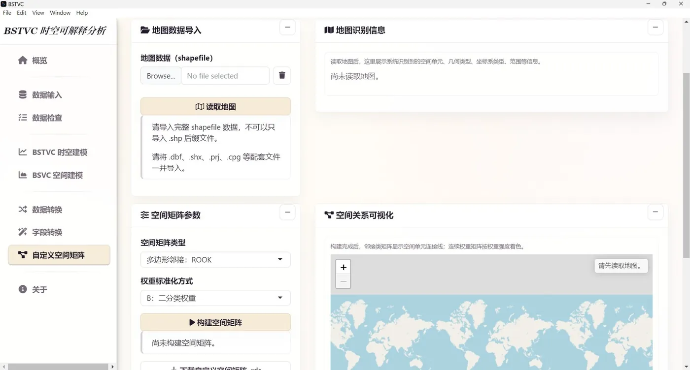
2000–2020 · 177 COUNTRIES AND TERRITORIES
SUITABLE FORExplaining why continuous indicators—such as life expectancy, resource quantities, concentrations, and rates—vary across places and periods.Gaussian likelihood on log-transformed response · identity link
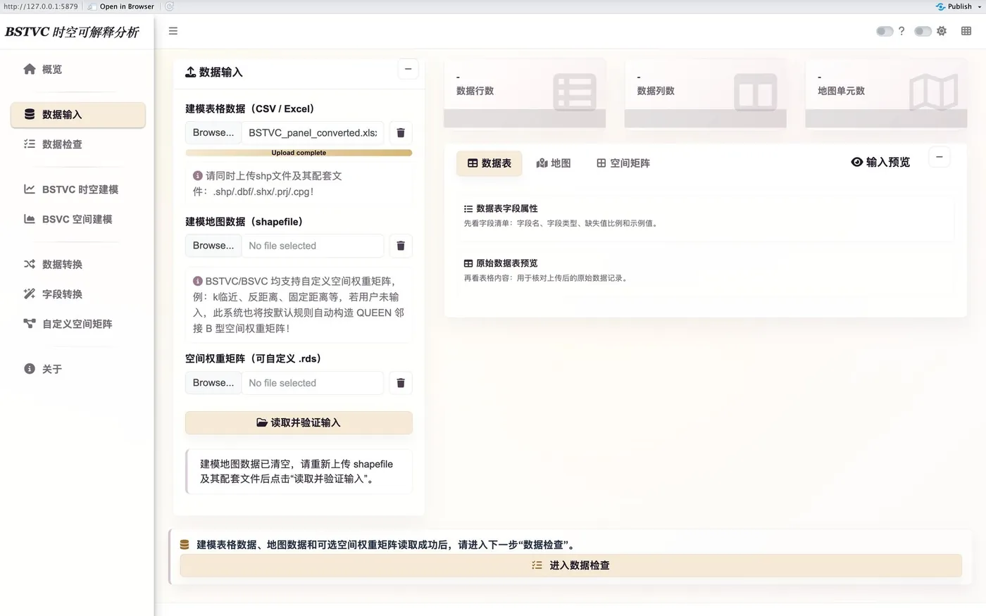
MONTHLY SPATIOTEMPORAL PANEL · 0/1 RESPONSE
SUITABLE FORStudying spatiotemporal determinants of 0/1 events such as disease occurrence, target attainment, or risk status.Bernoulli / Binomial likelihood · logit link
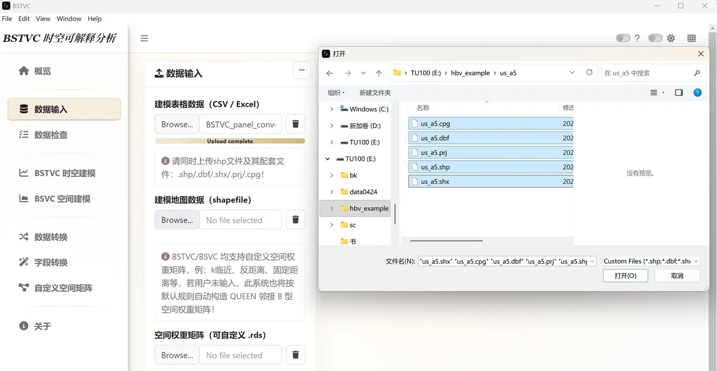
2012–2023 · U. S. SPATIAL UNITS
SUITABLE FORInvestigating local spatiotemporal mechanisms for non-negative count outcomes such as cases, events, or facilities.Poisson likelihood · log link
Do not treat strongly skewed or overdispersed counts, or 0/1 outcomes, as continuous variables. Transform data and inspect distributions when appropriate.
07 / READ THE OUTPUT
Do not interpret a coefficient in isolation. Combine TCs, SCs, STVPI, local predictions, credible intervals, and model assessment to build an interpretable conclusion.
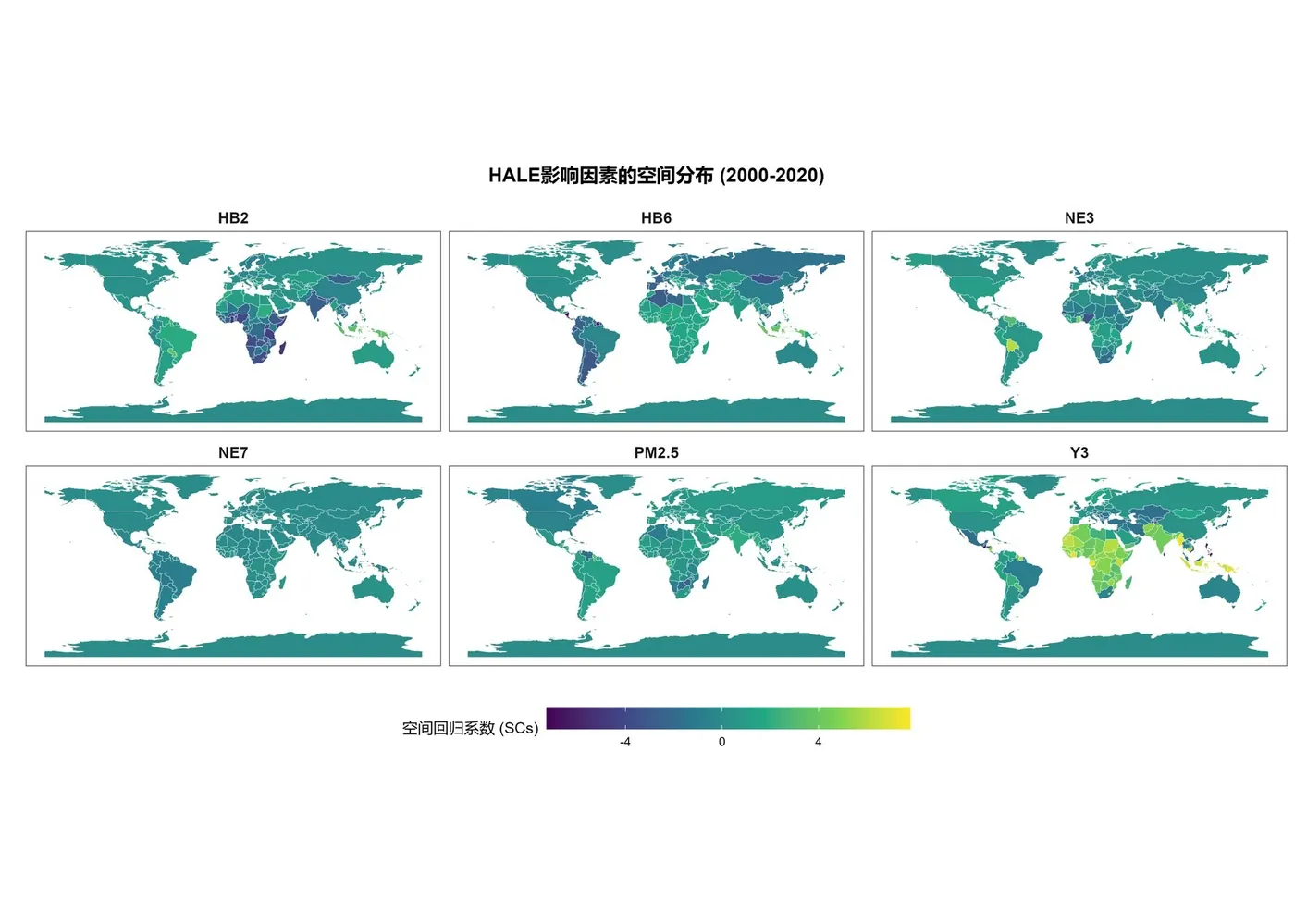
Spatial regression coefficients are exported by map unit for visualization in R, ArcGIS, ArcGIS Pro, or QGIS. Use consistent classes, color scales, and spatial extents across covariate maps.
RECOMMENDED: ArcGIS Pro / QGIS / R sfAssess direction and magnitude first, then the inner and outer credible intervals; finally integrate model assessment, mapped patterns, and substantive context.
Bayesian credible intervals express posterior parameter uncertainty and should not be mechanically equated with frequentist significance tests or reduced to significant/non-significant labels.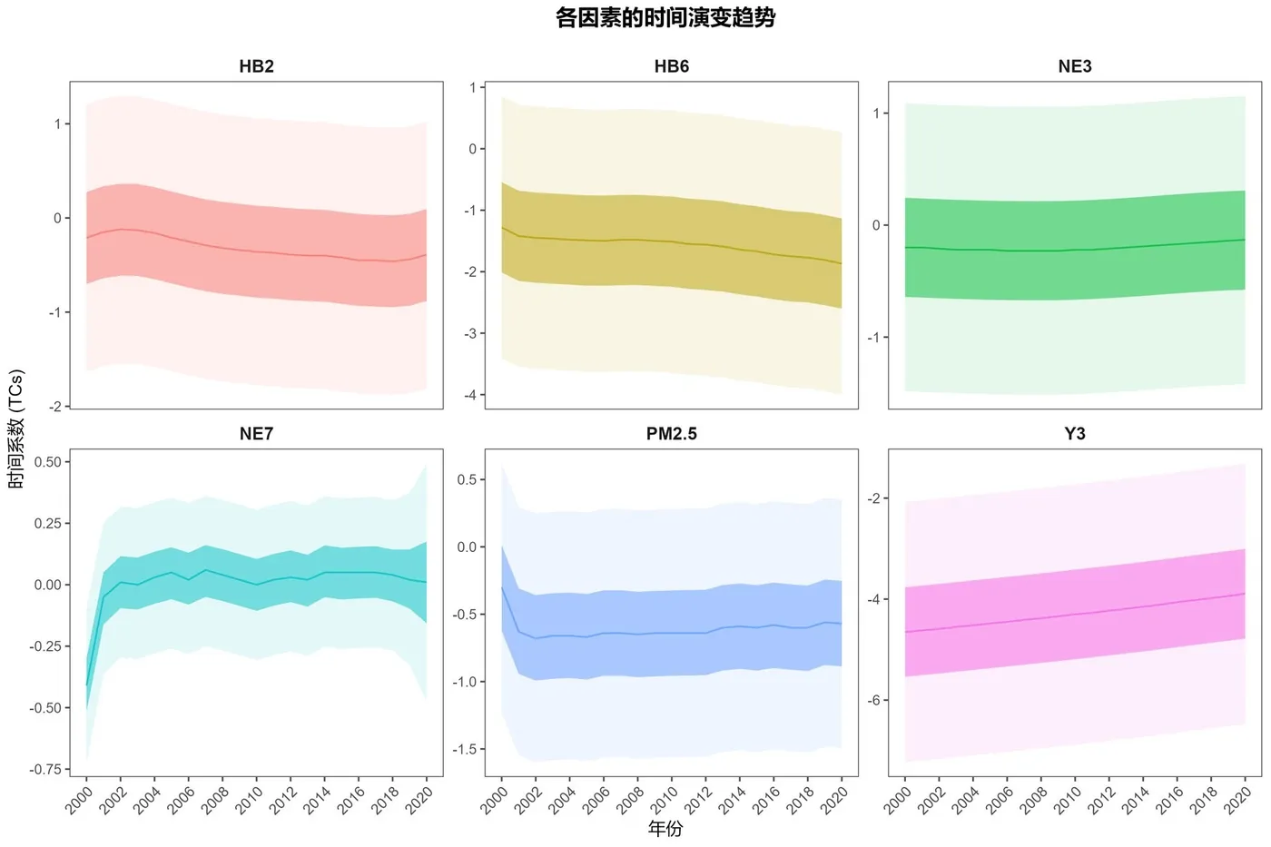
The mean curve represents the temporal regression coefficient; the darker band is the 50% credible interval and the lighter band is the 95% credible interval. Whether an interval crosses zero helps assess effect direction and evidential stability.
RECOMMENDED: R ggplot2 / ExcelAssess direction and magnitude first, then the inner and outer credible intervals; finally integrate model assessment, mapped patterns, and substantive context.
Bayesian credible intervals express posterior parameter uncertainty and should not be mechanically equated with frequentist significance tests or reduced to significant/non-significant labels.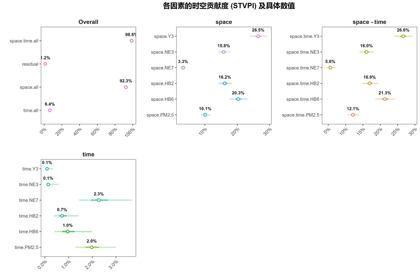
STVPI compares overall contributions and separates their temporal and spatial sources while retaining Bayesian uncertainty for key-driver identification.
RECOMMENDED: R ggplot2 / ExcelAssess direction and magnitude first, then the inner and outer credible intervals; finally integrate model assessment, mapped patterns, and substantive context.
Bayesian credible intervals express posterior parameter uncertainty and should not be mechanically equated with frequentist significance tests or reduced to significant/non-significant labels.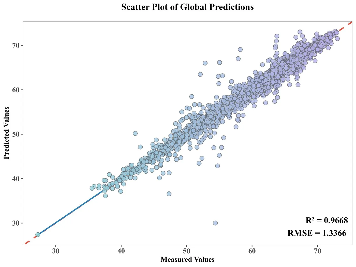
local. prediction contains observed y, imputed fill_y, model-based predict_y, and 50%/95% credible intervals, enabling R², RMSE, and response-specific performance metrics.
RECOMMENDED: R / ArcGIS Pro / ExcelAssess direction and magnitude first, then the inner and outer credible intervals; finally integrate model assessment, mapped patterns, and substantive context.
Bayesian credible intervals express posterior parameter uncertainty and should not be mechanically equated with frequentist significance tests or reduced to significant/non-significant labels.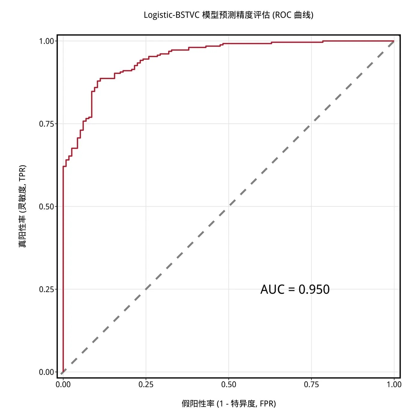
The ROC curve shows the trade-off between sensitivity and false-positive rate. A larger AUC generally indicates stronger discrimination and should be interpreted with local probability maps and uncertainty.
RECOMMENDED: R pROC / Python scikit-learnAssess direction and magnitude first, then the inner and outer credible intervals; finally integrate model assessment, mapped patterns, and substantive context.
Bayesian credible intervals express posterior parameter uncertainty and should not be mechanically equated with frequentist significance tests or reduced to significant/non-significant labels.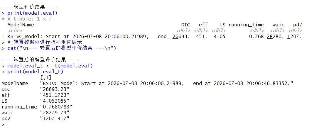
model. evaluation summarizes DIC, WAIC, eff, pd2, and LS. For candidate models, smaller DIC and WAIC usually indicate better fit; eff and pd2 reflect effective parameters and complexity; LS values closer to zero generally indicate better predictive accuracy.
RECOMMENDED: Excel / RAssess direction and magnitude first, then the inner and outer credible intervals; finally integrate model assessment, mapped patterns, and substantive context.
Bayesian credible intervals express posterior parameter uncertainty and should not be mechanically equated with frequentist significance tests or reduced to significant/non-significant labels.Lower values generally indicate better fit.
↓ LOWER IS GENERALLY BETTERQuantifies effective parameters and model complexity.
↔ INTERPRET WITH MODEL FITEvaluates accuracy and discrimination by response type.
LS → 0 · AUC ↑Reads temporal and spatial nonstationary effects separately.
DIRECTION + MAGNITUDE + CrI08 / SELECTED PUBLICATIONS
From methodological development to validation in health, social, and environmental settings, representative studies continue to test and extend the interpretive capabilities and application boundaries of the BSTVC model family.
Estimating Missing Values in China’s Official Socioeconomic Statistics Using Progressive Spatiotemporal Bayesian Hierarchical Modeling.
DOI ↗Exploring Spatiotemporal Nonstationary Effects of Climate Factors on Hand, Foot, and Mouth Disease Using Bayesian STVC.
DOI ↗Spatiotemporally Varying Coefficients Model: A Bayesian Local Regression to Detect Spatial and Temporal Nonstationarity.
DOI ↗Spatiotemporal Disparities in Regional Public Risk Perception of COVID-19 Using Bayesian STVC Series Models.
DOI ↗Spatiotemporal Heterogeneity in Associations of National Population Ageing with Socioeconomic and Environmental Factors.
DOI ↗Revealing Spatiotemporal Inequalities, Hotspots, and Determinants in Healthcare Resource Distribution.
DOI ↗09 / RESEARCH APPLICATIONS
Spatialized epidemiological odds ratios across 36 months in Sichuan to identify local seasonal trends and hotspots in disease–climate relationships.
Validated the general STVC formulation with ten years of county data and compared local spatiotemporal relationships between healthcare resources and socioeconomic conditions.
Revealed local environmental and socioeconomic effects on healthcare-resource inequality and produced a continuous county-level map series of hospital beds.
Compared globally stationary and locally nonstationary relationships using 30 candidate factors across 343 cities from 2008 to 2017.
Estimated the regional public risk perception index (PRPI) across 366 Chinese cities and performed cluster and outlier analysis.
Used STVC to identify local associations and STVPI to screen key drivers across 189 countries and territories over two decades.
Combined resource inequality, hotspot detection, and spatiotemporal determinants using a panel of hospital beds across 2,308 counties.
Characterized long-term MMR patterns at a small-area scale and examined heterogeneous effects of multilevel health determinants.
Compared spatiotemporal differences in resource patterns and socioeconomic effects across multiple urban healthcare-resource indicators in China.
Evaluated small-area spatiotemporal patterns and determinants of healthcare-resource allocation efficiency using a Sichuan county panel.
Extended research on local HFMD risk and driving mechanisms using a new spatiotemporally interpretable model.
Jointly characterized spatiotemporal changes in MMR and U5MR and connected dynamic prediction with interpretation of maternal and child health indicators.
For complete methods, original case figures, and updates, visit the BSTVC Model Homepage ↗
10 / FREE DOWNLOAD
English desktop release for Windows 10/11, with direct GitHub access to the installer, source repository, reproducible case interface, and supporting tools.
English installer · Windows x64 · Version 2026.8.1 · Released 1 August 2026
BSTVC_desktop_EN_win_x64_26.08.01_setup. exe SHA-2564f98423277254676d88eb64072e01920a597eaeddfaed1ee889bdcc0585c977c
Download from GitHub Release ↗
BSTVC-Desktop Repository
Releases, source, issue tracking, and version history
View GitHub Project ↗The module and integration point are reserved for the forthcoming English guide.
Coming soon · Link reservedReserved interface for example data, maps, and expected outputs
Future GitHub Release · Interface reservedCompare CPU, memory, and thread settings locally
View GitHub Project ↗https://pan.baidu.com/s/5h7zSPjXEvBINShxLVLjirA
11 / USER GUIDE KNOWLEDGE HUB
Use the tabs to navigate data preparation, nine parameters, six output types, current limitations, R-package installation, documentation, and support.
Supports CSV, XLSX, and XLS. Import the complete Shapefile set rather than a standalone. shp file.
The spatial-unit order in every time slice must match the map. The desktop app can compare, reorder, and export validated data automatically.
The table and map must use spatial identifiers with matching names and types; represent missing values consistently as NA.
Built-in data conversion, field conversion, and custom spatial matrices support wide-to-long reshaping and numeric field conversion.
Choose Original Data if spatial order is unchanged; choose Validated Data after automatic reordering.
Specify response Y, one or more explanatory variables X, the Time field, and the Space field.
Choose continuous, binary, or count according to the data; each response type uses a different likelihood.
Standardize explanatory variables where appropriate. The default is six threads; spatial weights can use QUEEN-B or a custom matrix.
Model fit, complexity, and predictive assessment using DIC, WAIC, eff, pd2, and LS.
Local predictions, missing-value imputations, and 50%/95% Bayesian credible intervals.
Spatial and temporal random effects for explanatory variables, with corresponding credible intervals.
Temporal coefficients, spatial coefficients, and relative spatiotemporal contribution percentages, downloadable as a multi-sheet Excel workbook.
The upload limit is 1 GB. Computational demand increases with spatial units, time points, explanatory variables, response type, and thread settings.
For point maps, use distance-based or k-nearest-neighbor matrices. If a kNN matrix triggers an INLA error, adjust its construction or use another matrix type.
The current binary and count models do not include a residual term, so an overall explained-percentage metric is not yet available.
BSTVC currently assumes spatiotemporal nonstationarity for all explanatory variables; more flexible variable-level settings are planned.
bayesianstvc/BSTVC-R supports continuous, binary, and count responses within a full-map framework, producing local mechanisms, key-driver evidence, and dynamic predictions.
The current README uses devtools:: install_github("songbi123/BSTVC") or remotes:: install_github("songbi123/BSTVC"); install INLA first according to its official instructions.
DESCRIPTION specifies R ≥ 4.4.0 and INLA ≥ 24.06.27 under GPL-3; model assessment covers DIC, WAIC, pd, and LS.
The repository provides GetStart. Rmd, English and Chinese PDFs, preprocessing scripts, and GitHub Issues. Desktop supports no-code reproduction; the R package supports batch research.
Source, releases, installation, and Issues.
CHINESE GUIDE / PDFChinese User Guide ↗Data, modeling, outputs, and visualization.
ENGLISH GUIDE / PDFGetStart-English ↗R-package examples and reproducible workflows.
DEPENDENCY / INLAINLA Installation Guide ↗Dependencies and version notes for large Bayesian computations.
MODEL / HOMEPAGEBayesian STVC Model Homepage ↗Theory, methodological evolution, and research cases.
TOOL / MONITORBSTVC Process Monitor ↗Monitor CPU, memory, and thread settings.
12 / AUXILIARY TOOL
 BSTVC
BSTVCA lightweight resource monitor for BSTVC Desktop that tracks CPU, memory, and thread states during model computation to support faster, more stable settings.
Different data scales, model structures, and hardware configurations have different resource sweet spots. Start with the BSTVC default of six threads, then compare eight or 12 using real trajectories from similar models.
Start with the default six threads, then adjust using monitor results from comparable models.
Monitor one or more inla. exe processes and continuously record system-wide CPU, memory, threads, PID, runtime, and status. The main CPU series matches the system-wide metric shown by Windows Task Manager.
More threads are not always faster. Balance sustained CPU activity, memory pressure, variability, and solve time for your computer or workstation; the default remains six threads.
The monitor runs locally through PowerShell and a browser, requires no cloud service, and uploads no process data. Each run can save CSV, JSON, and local HTML reports.
Start with the default six threads. Try eight threads only when memory is sufficient and the task is large. Reserve 12 threads for many-core, high-memory systems and confirm stable headroom with the monitor.
Published by bayesianstvc. Runs on Windows 10/11 with PowerShell 5.1 or 7 and a modern browser. View v0.5.7 Release ↗
13 / CONTACT & FEEDBACK
Project lead, statistical-methodology advisor, and copyright holder.
chaosong.gis@gmail.com ↗Software developer responsible for system design and user support.
tangxt.me@gmail.com ↗
BSTVC ORGANIZATION
Bayesian Spatiotemporally Varying Coefficients
BSTVC Desktop · Data preparation, model configuration, and result export
